Getting Started

Want to follow along? Download this notebook.

Performing a QEC experiment with Deltakit typically involves four steps.

1. In the circuit generation step, you generate a quantum circuit to implement the experiment of interest, such as quantum memory or stability. In this step, you compile a noisy physical circuit based on your QPU’s native gates and their characteristics.

2. In the simulation step, you simulate the circuit using Stim.

3. In the decoding step, you choose a decoder to decode your measurement results. You can use both open-source decoders, like minimum weight perfect matching (MWPM), and propriety decoders, like Ambiguity Clustering (AC).

4. In the analysis step, you interpret the results of your QEC experiment, and calculate and visualise the logical error probability and error suppression factor \(\Lambda\).

Circuit Generation

Idealised Circuit

To generate the underlying circuit for quantum memory experiments, there are several common quantum error correction codes you can use, including:

• Rotated planar codes (RotatedPlanarCode),

• Unrotated planar codes (UnrotatedPlanarCode),

• Unrotated toric codes (UnrotatedToricCode),

• Repetition codes (RepetitionCode),

• Bivariate bicycle codes (BivariateBicycleCode), and

• (More generally) any CSS code (CSSCode).

To get the logical error probability with a quantum memory experiment, for example, you can use the rotated planar code to encode a logical qubit:

from deltakit.explorer import codes
# configure the rotated planar code
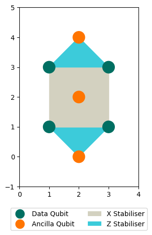
code = codes.RotatedPlanarCode(width=2, height=2)
code.draw_patch()

(<Figure size 640x480 with 1 Axes>, <Axes: >)

You can then pass this code to the css_code_memory_circuit function to generate a noiseless circuit for a quantum memory experiment, for example, using a single round and measuring in the logical Pauli Z basis:

from deltakit.explorer.codes import css_code_memory_circuit
from deltakit.circuit.gates import PauliBasis

circuit = css_code_memory_circuit(code, num_rounds=1, logical_basis=PauliBasis.Z)

This returns a Circuit object, which contains the quantum circuit that encodes a memory experiment using the error correcting code you chose in the first cell.

circuit

Circuit([
    GateLayer([
        RZ(Qubit(Coord2D(3, 1)))
        RZ(Qubit(Coord2D(1, 1)))
        RZ(Qubit(Coord2D(3, 3)))
        RZ(Qubit(Coord2D(1, 3)))
        RX(Qubit(Coord2D(2, 0)))
        RX(Qubit(Coord2D(2, 2)))
        RX(Qubit(Coord2D(2, 4)))
    ])
    GateLayer([
        I(Qubit(Coord2D(1, 1)))
        I(Qubit(Coord2D(1, 3)))
        I(Qubit(Coord2D(3, 1)))
        I(Qubit(Coord2D(3, 3)))
    ])
    GateLayer([
        CZ(control=Qubit(Coord2D(2, 0)), target=Qubit(Coord2D(1, 1)))
        CX(control=Qubit(Coord2D(2, 2)), target=Qubit(Coord2D(1, 3)))
    ])
    GateLayer([
        CZ(control=Qubit(Coord2D(2, 0)), target=Qubit(Coord2D(3, 1)))
        CX(control=Qubit(Coord2D(2, 2)), target=Qubit(Coord2D(1, 1)))
    ])
    GateLayer([
        CX(control=Qubit(Coord2D(2, 2)), target=Qubit(Coord2D(3, 3)))
        CZ(control=Qubit(Coord2D(2, 4)), target=Qubit(Coord2D(1, 3)))
    ])
    GateLayer([
        CX(control=Qubit(Coord2D(2, 2)), target=Qubit(Coord2D(3, 1)))
        CZ(control=Qubit(Coord2D(2, 4)), target=Qubit(Coord2D(3, 3)))
    ])
    GateLayer([
        MX(Qubit(Coord2D(2, 0)), probability=0.0)
        MX(Qubit(Coord2D(2, 2)), probability=0.0)
        MX(Qubit(Coord2D(2, 4)), probability=0.0)
        MZ(Qubit(Coord2D(3, 1)), probability=0.0)
        MZ(Qubit(Coord2D(1, 1)), probability=0.0)
        MZ(Qubit(Coord2D(3, 3)), probability=0.0)
        MZ(Qubit(Coord2D(1, 3)), probability=0.0)
    ])
    Detector([MeasurementRecord(-7)], coordinate=Coordinate(np.int64(2), np.int64(0), 0))
    Detector([MeasurementRecord(-5)], coordinate=Coordinate(np.int64(2), np.int64(4), 0))
    ShiftCoordinates(Coordinate(0, 0, 1))
    Observable([MeasurementRecord(-3), MeasurementRecord(-1)], index=0)
    Detector([MeasurementRecord(-7), MeasurementRecord(-4), MeasurementRecord(-3)], coordinate=Coordinate(np.int64(2), np.int64(0), 0))
    Detector([MeasurementRecord(-5), MeasurementRecord(-1), MeasurementRecord(-2)], coordinate=Coordinate(np.int64(2), np.int64(4), 0))
    ShiftCoordinates(Coordinate(0, 0, 1))
], iterations=1)

To convert the circuit to stim, you can run:

stim_circuit = circuit.as_stim_circuit()

which is then easy to visualise:

stim_circuit.diagram(type="timeline-svg")

Realistic Circuit

You can now add a noise model and compile the circuit into the native gate set of a realistic QPU.

Noise

To simulate a realistic noise environment on a QPU, you can use several common noise models with deltakit.explorer.qpu, including:

• Phenomenological noise (PhenomenologicalNoise), which uses a fixed probability of depolarisation after each gate;

• Standard depolarising noise (SD6Noise), which has a single probability of incorrect measurement and depolarisation after each gate, idle cycle, and reset operation;

• “Toy” noise (ToyNoise), which parametrizes the probabilities of incorrect measurement and depolarisation after gate and idle cycle with two parameters; and

• SI1000 noise (SI1000Noise), a noise model inspired by superconducting qubits.

For example:

from deltakit.explorer.qpu import SI1000Noise
noise_model = SI1000Noise(p=1e-3)  # 0.001 physical error rate

You can also configure more general noise models using NoiseParameters.

Native Gates

With Deltakit, you can define a QPU’s native gate set by specifying its one qubit, two qubit, reset, and measurement gates.

from deltakit.explorer.qpu import NativeGateSet
from deltakit.circuit.gates import SQRT_X, SQRT_X_DAG, S_DAG, S, X, Z, CZ,RZ, MZ
native_gates = NativeGateSet(
    one_qubit_gates={SQRT_X, SQRT_X_DAG, S_DAG, S, X, Z},
    two_qubit_gates={CZ},
    reset_gates={RZ},
    measurement_gates={MZ},
)

With the noise model and native gate set defined, you can now generate an object to represent the QPU object, and compile your circuit to simulate the target QPU.

from deltakit.explorer.qpu import QPU
qpu = QPU(qubits=code.qubits,
          native_gates_and_times=native_gates,
          noise_model=noise_model)
qpu_circuit = qpu.compile_and_add_noise_to_circuit(circuit)
qpu_circuit.as_stim_circuit().diagram(type="timeline-svg")

With the noisy, qpu-native circuit generated, you’re now ready to tackle the next step of your quantum error correction experiment: simulation.

Simulation

To sample raw output from the circuit, you can use stim features directly:

1. Convert to stim circuit

2. Compile a stim “sampler” from the circuit

3. Sample using the sampler

stim_circuit = qpu_circuit.as_stim_circuit()  # 1
sampler = stim_circuit.compile_sampler()  # 2
sampler.sample(shots=3)  # 3

array([[ True,  True,  True,  True,  True,  True,  True],
       [ True,  True,  True, False, False, False, False],
       [ True,  True,  True, False, False, False, False]])

The output is a boolean NumPy array representing the seven measurement outcomes for three separate shots.

Typically, the focus is not on the individual measurement outcomes but on logical errors. Assessing those is the job of the decoder.

Decoding

Deltakit currently exposes one decoder for use locally, PyMatching. (However, there are many other decoder options when using the remote workflow, and there are many local decoder analysis and manipulation tools in deltakit.decode.)

(PyMatchingDecoder.construct_decoder_and_stim_circuit) is a helper factor that accepts a circuit and returns two things:

• an object representing a Minimum Weight Perfect Matching decoder and

• a modified version of the original circuit configured to operate with the decoder.

from deltakit.decode import PyMatchingDecoder
decoder, decoder_circuit = PyMatchingDecoder.construct_decoder_and_stim_circuit(qpu_circuit)

(run_decoding_on_circuit) accepts these objects and the maximum number of shots to sample, returning a dictionary that contains the actual number of shots and the number of failures (shots for which the decoder incorrectly assessed whether the observable had flipped or not).

from deltakit.decode.analysis import run_decoding_on_circuit
results = run_decoding_on_circuit(decoder_circuit, 1000, decoder)
print(f"There were {results['fails']} failures out of {results['shots']} shots.")

  0%|          | 0/1 [00:00<?, ?it/s]

Shots: 1000; Fails: 14; RSE: 0.265:   0%|          | 0/1 [00:00<?, ?it/s]

Shots: 1000; Fails: 14; RSE: 0.265: 100%|██████████| 1/1 [00:00<00:00, 415.77it/s]

There were 14 failures out of 1000 shots.

To scale beyond simple experiments, it is useful to define the concept of a “Decoder Manager”, which represents the combined experiment circuit and decoder system. The StimDecoderManager accepts the circuit and decoder objects and returns a decoder manager. Similar to the run_decoding_on_circuit function, its run_batch_shots method returning the total number of shots and the number of failures.

from deltakit.decode.analysis import StimDecoderManager
decoder_manager = StimDecoderManager(decoder_circuit, decoder)
n_shots, n_fails = decoder_manager.run_batch_shots(1000)
print(f"There were {n_fails} failures out of {n_shots} shots.")

There were 24 failures out of 1000 shots.

Analysis

Deltakit also provides tools for summarising the results of experiments. To calculate the LEP (Logical Error Probability) and its standard error, use the calculate_lep_and_lep_stddev function.

from deltakit.explorer.analysis import calculate_lep_and_lep_stddev
lep, lep_stddev = calculate_lep_and_lep_stddev(
    fails=[n_fails],
    shots=[n_shots],
)
print(f"LEP: {lep[0]}, LEP std: {lep_stddev[0]}")

# confirm the calculation manually
import numpy as np
from scipy import stats
lep0 = n_fails / n_shots
lep_stddev0 = stats.sem([1]*n_fails + [0]*(n_shots - n_fails), ddof=0)
np.testing.assert_allclose(lep, lep0)
np.testing.assert_allclose(lep_stddev, lep_stddev0)

LEP: 0.024, LEP std: 0.004839834707921336

Now you can start varying different parameters to see how that changes the logical error probability, such as the code distance. You can pass a list of decoder managers and number of shots to RunAllAnalysisEngine, and use the run method to run your simulations. This method then returns a dataframe that summarises the results.

from deltakit.decode.analysis import RunAllAnalysisEngine

distances = [5, 7, 9]
all_shots, all_fails = [], []
decoder_managers = []
for d in distances:
    code = codes.RotatedPlanarCode(width=d, height=d)
    circuit = css_code_memory_circuit(code, num_rounds=d, logical_basis=PauliBasis.Z)
    qpu = QPU(qubits=code.qubits, native_gates_and_times=native_gates, noise_model=noise_model)
    qpu_circuit = qpu.compile_and_add_noise_to_circuit(circuit)
    decoder, decoder_circuit = PyMatchingDecoder.construct_decoder_and_stim_circuit(qpu_circuit)
    decoder_managers.append(StimDecoderManager(decoder_circuit, decoder))

engine = RunAllAnalysisEngine("my experiment", decoder_managers=decoder_managers, max_shots=100000)
df = engine.run()
df['distance'] = distances
df

Evaluating codes:   0%|          | 0/3 [00:00<?, ?it/s]

Evaluating codes:  33%|███▎      | 1/3 [00:00<00:01,  1.12it/s]

Evaluating codes:  67%|██████▋   | 2/3 [00:03<00:01,  1.87s/it]

Evaluating codes: 100%|██████████| 3/3 [00:08<00:00,  3.32s/it]

Evaluating codes: 100%|██████████| 3/3 [00:08<00:00,  2.83s/it]

	decoder	noise_name	shots	fails	distance
0	MWPM	SampleStimNoise	100000	143	5
1	MWPM	SampleStimNoise	100000	29	7
2	MWPM	SampleStimNoise	100000	8	9

calculate_lep_and_lep_stddev can calculate all the logical error probabilities in batch.

from deltakit.explorer.analysis import calculate_lep_and_lep_stddev
leps, leps_std = calculate_lep_and_lep_stddev(df['fails'], df['shots'])
df['LEP'] = leps
df['LEP std'] = leps_std
df

	decoder	noise_name	shots	fails	distance	LEP	LEP std
0	MWPM	SampleStimNoise	100000	143	5	0.00143	0.000119
1	MWPM	SampleStimNoise	100000	29	7	0.00029	0.000054
2	MWPM	SampleStimNoise	100000	8	9	0.00008	0.000028

To estimate the error scaling parameter \(\Lambda\), use the calculate_lambda_and_lambda_stddev function:

from deltakit.explorer.analysis import calculate_lambda_and_lambda_stddev
res = calculate_lambda_and_lambda_stddev(distances, leps, leps_std)
res.lambda_

4.52209939569218

Now that you have an overview of the four steps of QEC experimentation with Deltakit, please continue with the following guides.

• Authentication
• QEC Experiment Circuit Generation
• Adding Noise
• Simulation
• Decoding
• Quantum Error Correction Analysis Tools
• Error budgeting for quantum error correction